Multi-Armed Bandit Agents

Introduction to Multi-Armed Bandits

In Reinforcement Learning, there is typically a goal-directed agent that seeks to explore its interaction with the environment, guided by rewards. In this simulation, agents are equipped with various action-selection rules (ASRs). These ASRs are modeled as a map called policy. The idea is to explore the actions in the state space, observe and record the best actions (via quantified reward response to said action), and ultimately, balance exploration with exploitation. The following is a (hopefully) intuitive approach to understanding the exploration-vs-exploitation dilemma in reinforcement learning.

Agent action selection rules:

• Greedy Approach
• Plan: always choose the action with the highest rewarded return. (i.e. The one that looks best at present).
• Problem: purely exploitative. No exploration! So, it relies on luck to get it right from the start. We'd like some guarentee, in the limit, to find the optimal policy
• Epsilon-Greedy Approach
• Plan: At each trial, randomly choose (or sample) an action with the probability 𝜖 (epsilon), otherwise, exploit the current best action with the greedy choice with probability 1-𝜖
• Problem: Well, we don't know when to stop exploring (i.e. when we've found the best action).
• Epsilon-First Approach
• Plan: For the initial n trials, randomly sample the actions. Then, use the greedy policy.
• Problem: (1) Don't know how much time to spend sampling (how to pick n). (2) All the 'static' sampled actions don't ensure that we've found the optimal arm, there could be a better option. (3) The time used exploring could be wasted, causing an accumulation of regret!
• Epsilon-Decreasing Approach
• Simulated Annealing: a slow decrease in the probability of accepting worse solutions as the solution space is explored.
• Plan: Modify the 𝜖-greedy approach to decreasing epsilon over time using a cooling schedule.
• Problem: Still aren't sure about if we may be annealing too fast to miss exposure to the best option, or too slow and miss rewards, accumulating regret.

Summary of ASRs

MAB represents a sequential decision problem: initially unknown reward distributions associated with each arm/choice. Remember, we have treated each arm like a unique slot machine- we'd like to find the best machine to play with our finite cash & time.

The idea is: we need some way to model uncertainty of what the "true" reward rates of each slot machine arm are! We know, thanks to the Law of Large Numbers, that as we take more and more samples, we have less uncertainty.

Thompson Sampling Explained

We know that there is some unknown, but "fixed" probability of reward for each action/arm. Using Probability Density Functions, we use area/distribution over possible likelihoods that have less variance the more samples are collected. We represent our belief in the best action by fitting some PDF to estimate this true reward, where PDFs can be sampled from to obtain a possible probability. Therefore, the more an arm is chosen/sampled, the closer the PDF P(R|a) is to its true probability, where R ∈ {0,1} ∀ arms a.

In other words, the curves of options are estimates of reward. Random choice/sample refines confidence in expectation of the reward/outcome probability

Understanding Upper Confidence Bound

Despite the elegant representation of the options, there still will be uncertainty about the accuracy of the action-value estimates. Plus, the environment may be dynamic, adapting to our experience live. Online learning like this is orders of magnitude harder.

The greedy actions take the seemingly best actions in the present moment. So, we need exploration. Epsilon greedy action forces non-greedy actions to be tried, but indiscriminately, with no preference for the nearly greedy or particularly uncertain, mysterious actions. It would behoove us to take these aspects into account, selecting near-greedy actions according to their potential for being the optimal choice.

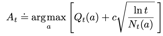
Here, we can say that the action for Upper Confidence Bound (UCB) should be the argmax (a value at a at which f(a) takes its maximal value of the expression that follows). ln t denotes the natural logarithm of t (the number that e ≈ 2.71828 would have to be raised to in order to equal t), Nt(a) denotes the number of times that action a has been selected prior to time t (the denominator), and the number c > 0 controls the degree of exploration. If Nt(a) = 0, then a is considered to be a maximizing action

The idea is that the upper confidence bound action selection method is that the square root term is a measure of the uncertainty of a's value, with c determining the confidence level. We want to 'max' over the true value of action a. When a is selected, the Nt(a) increments, and as it is in the denominator, decreasing the uncertainty term. Using natural logarithm means that the increases get smaller over time, but are unbounded; all actions will eventually be selected, but actions with lower value estimates, or that hvae already been selected frequently, will be selected with decreasing frequency over time.