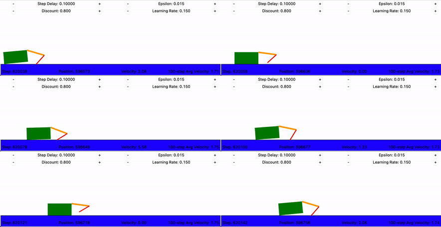
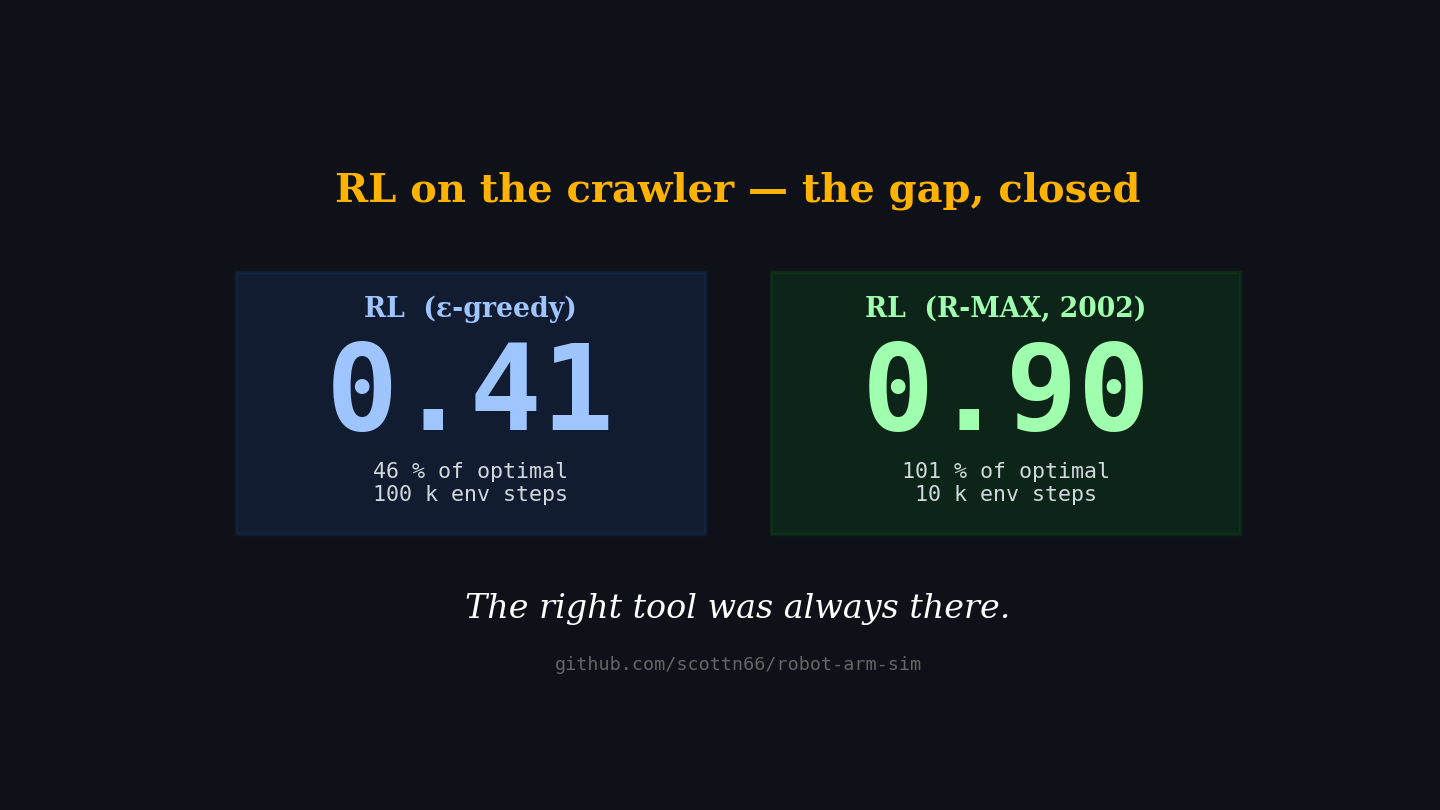
A two-jointed robot teaches itself to crawl. We spent a small eternity tuning the reinforcement-learning recipe, and reached only 42% of optimal. Then a single algorithm from 2002 closed the gap to 100%. Here's the whole story.
The optimal gait, discovered online by R-MAX, verified against dynamic programming.
The crawler is a classic UC Berkeley CS188 environment: a body on a wheel, an arm, and a hand. Four buttons, arm up/down, hand up/down. Push them in the right order and the body ratchets forward. The agent gets a reward equal to how far it moved each step. It has no body diagram, no physics model. Just trial and error.
We threw an escalating stack of reinforcement-learning machinery at it: ε-greedy schedules, cross-validated decay sweeps, Bayesian optimization, population-based training, evolutionary refinement, scaling laws, a from-scratch DQN, reward shaping, count-based exploration. Every method converged to roughly the same ceiling: a peak velocity around 0.41.
We never knew that was only 42% of optimal, because we'd never computed the optimum. The crawler is a finite, deterministic Markov Decision Process. You can solve it exactly with dynamic programming in about three seconds, using an algorithm from 1957. When we finally did, the optimal policy crawled 2.4× faster than anything reinforcement learning had produced. The fix wasn't more tuning, it was a different class of algorithm.
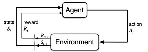
A Markov Decision Process is a deceptively simple model: an agent observes a state, takes an action, receives a reward, and lands in a new state. The subscript t on each arrow marks a step in time, much like taking a turn in a board game.
Q-Learning is a model-free reinforcement-learning algorithm: it learns the expected long-run value of each (state, action) pair without ever building a model of the environment. It works by repeatedly applying the Bellman update:
$Q(s, a) \leftarrow Q(s, a) + \alpha\,\big[\,r + \gamma \max_{a'} Q(s', a') - Q(s, a)\,\big]$
where $\alpha$ is the learning rate, $\gamma$ the discount factor, $r$ the reward, and $s'$ the next state. Background reading:
Agent SARSA TD learning Bellman equation
Continually updating Q-values lets the agent converge, in principle, to the optimal policy for any finite MDP. The question this project asks is: how close does it actually get, and how fast?
Each technique below was a genuine attempt to push past the ceiling. Each one is a different idea from the RL literature. None of them broke through - because they're all model-free: they optimize how the agent explores or approximates, never what it knows about the world.
schedule sweeps Bayesian optimization population-based training evolutionary refinement scaling laws DQN reward shaping count-based exploration
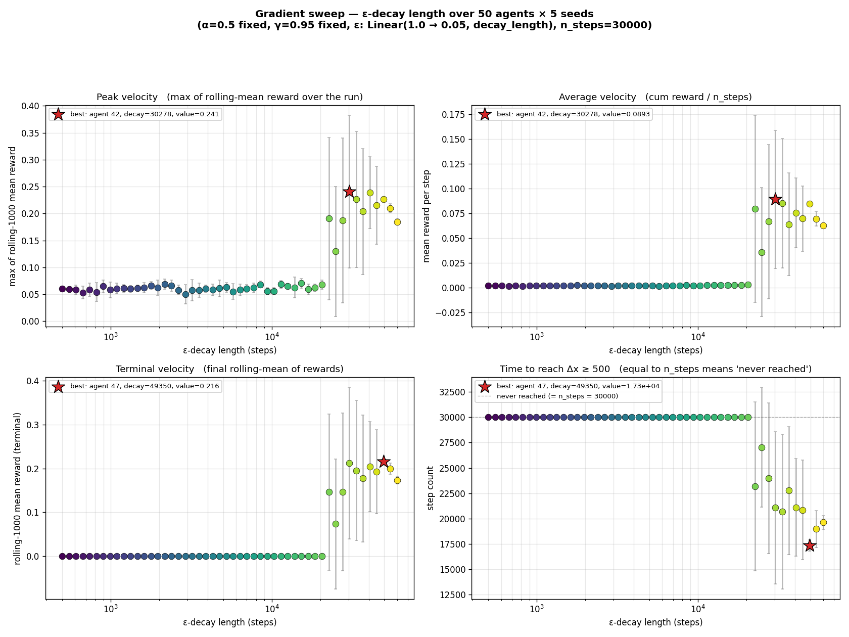
Each of the four panels measures the same 50 trained agents along a different axis of performance:
X-axis (all four): ε-decay length on a log scale, how many steps
ε took to anneal from 1.0 (pure random) down to 0.05 (near-greedy).
Dot color: each agent's position on the gradient (viridis: deep
purple = shortest decay, bright yellow = longest).
Error bars: ±1 standard deviation across 5 random seeds
per agent. The simulator itself is deterministic given a seed, but the
seed sets the initial Q-table and the ε-greedy coin flips, so different
seeds find different paths to (or away from) the optimum.
Red star: the agent whose mean across seeds was best on
that panel's metric.
We even found that the "right" amount of exploration isn't a property of the task, it shifts with the learning rate and discount factor. Interesting science, but all of it within the same basin of attraction at 42% of optimal.
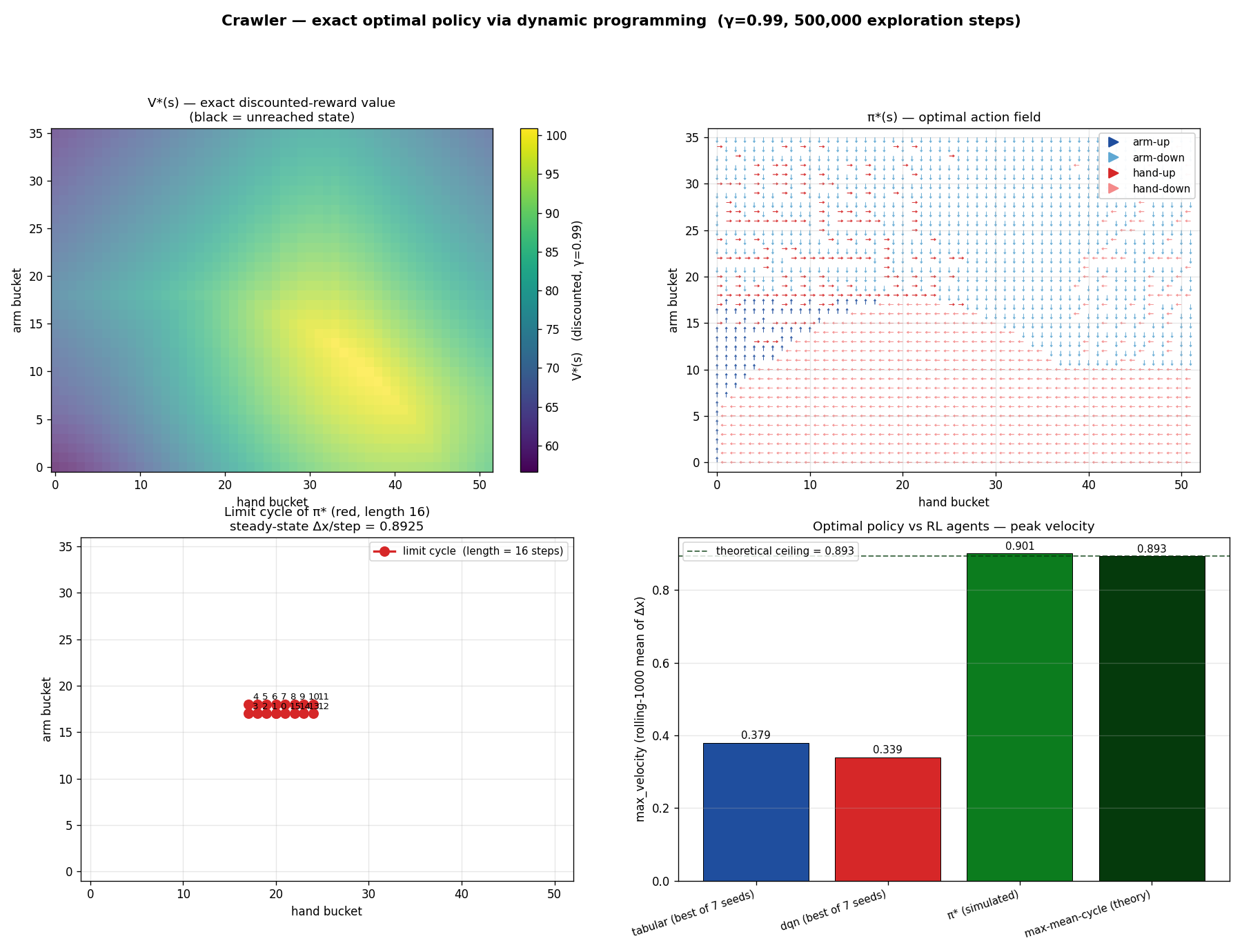
Because the crawler is a deterministic finite MDP, we can build its transition table exhaustively, run value iteration until $V^*(s)$ converges, and read off the optimal policy. Total compute: about three seconds. We cross-checked with Karp's max-mean-cycle algorithm (1978) for the true asymptotic velocity ceiling. They agree.
| approach | peak velocity | % of optimum |
|---|---|---|
| π* via value iteration | 0.901 | 100% |
| Karp max-mean-cycle (theory) | 0.894 | 99% |
| best tabular Q-learning | 0.379 | 42% |
| best DQN | 0.340 | 38% |
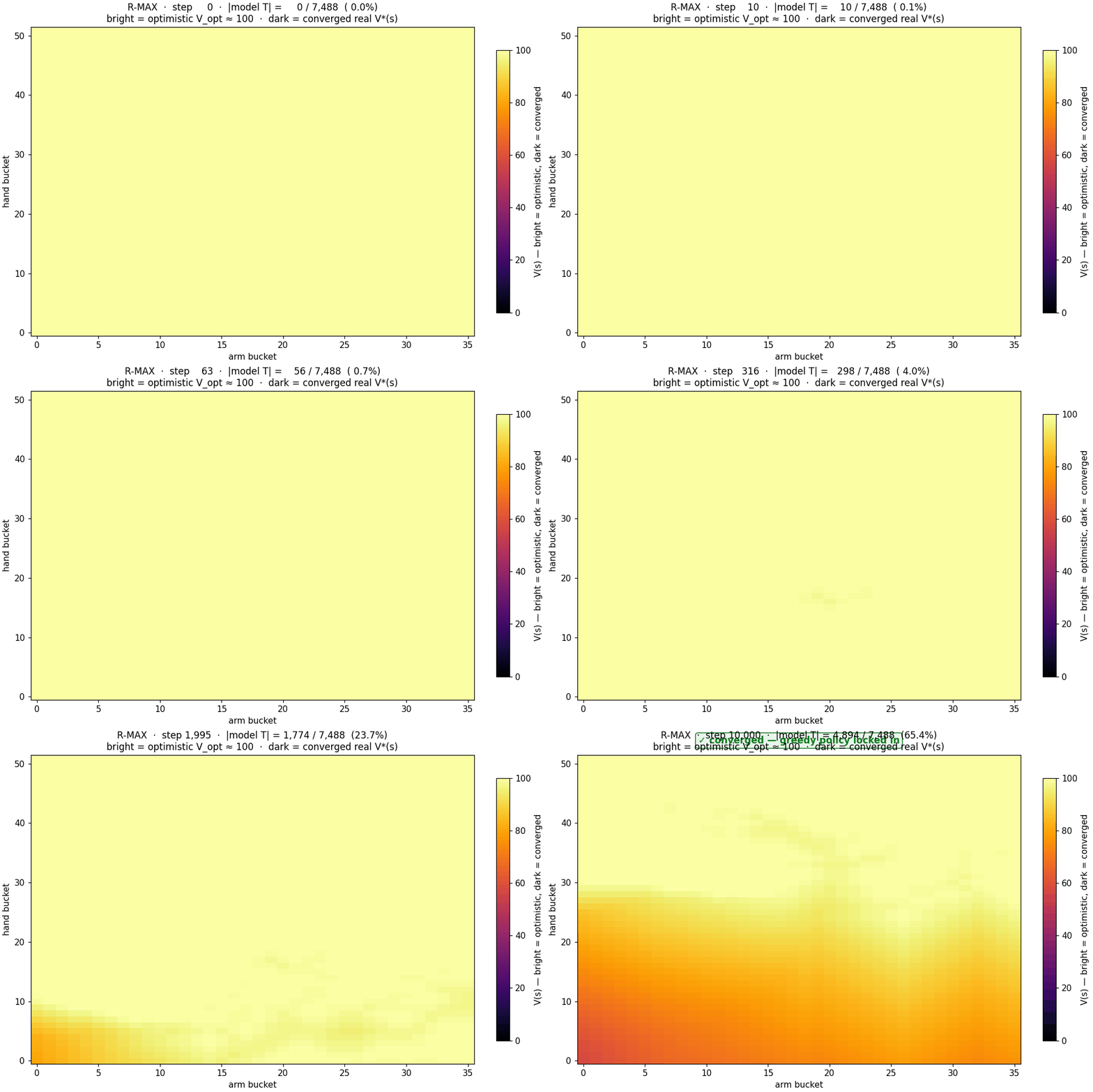
The fix was in the literature all along. Brafman & Tennenholtz's R-MAX (2002) is still reinforcement learning, the agent has no model handed to it, but it builds one from experience and plans with it. Its trick is optimism under uncertainty: any state-action pair it hasn't tried is assumed to pay the maximum possible reward forever. That assumption mathematically forces the agent toward unexplored corners, no ε-schedule, no exploration heuristic required.
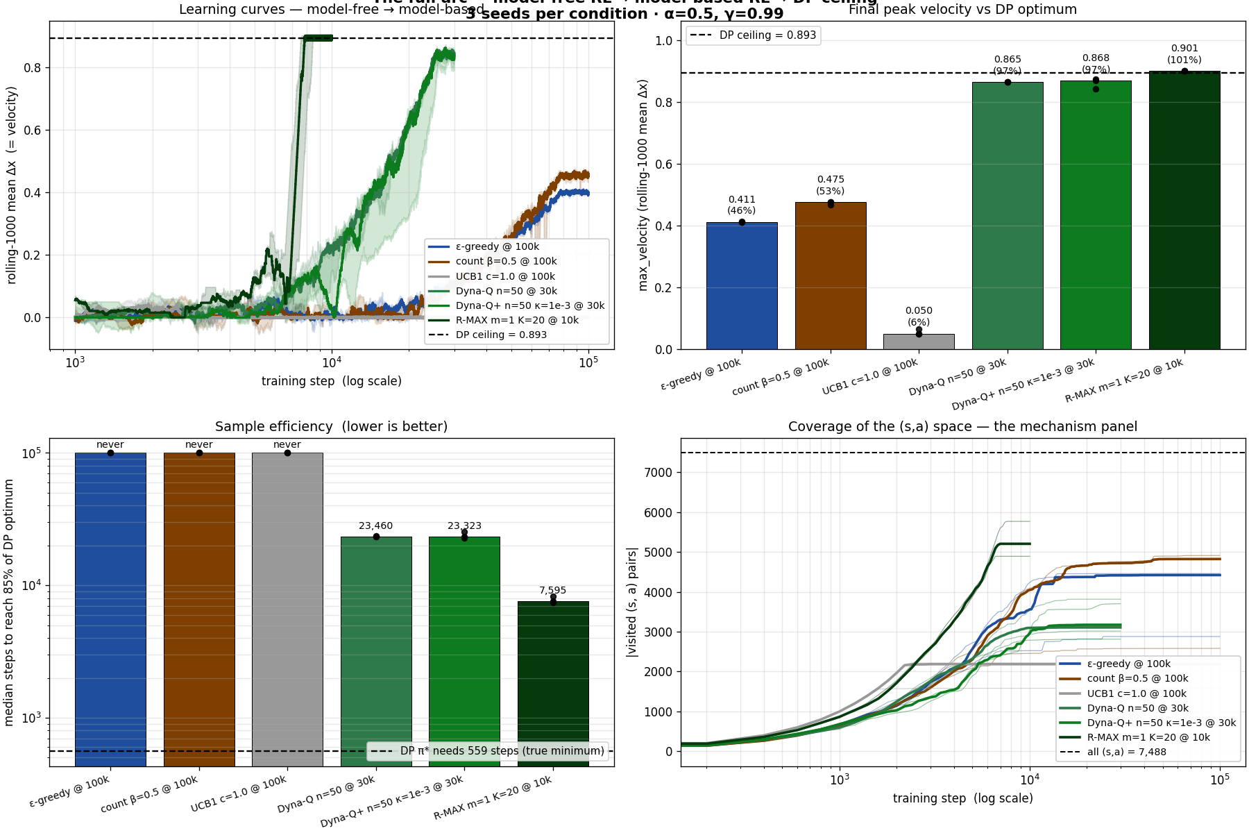
Dyna-Q (bare model + planning, no exploration trick) already reaches 97% of optimal. R-MAX reaches 101%, within seed noise of the DP ceiling, in fewer environment steps than vanilla Q-learning needs to start moving.
The bar chart says it numerically. The race says it viscerally:
The lesson isn't "RL is bad." It's that the right axis of choice is model-free vs model-based, not which exploration trick or which optimizer. Model-free RL earns its keep on problems too big to enumerate (Atari, robotics with messy contact dynamics). The crawler isn't that. And the surprise is that even here, RL can match dynamic programming, as long as you let it learn the model.
Everything is reproducible from the repo:
git clone https://github.com/scottn66/robot-arm-sim.git
cd robot-arm-sim
pip install matplotlib scikit-learn scipy numpy pillow
# Live GUI (watch the optimal schedule crawl in real time)
python3 src/crawler.py
# Compute the exact optimum (value iteration + Karp's cycle)
python3 scripts/find_optimal_policy.py
# The full algorithm-spectrum comparison: epsilon-greedy -> R-MAX
python3 scripts/compare_full_arc.py